Relevant to ACCA Qualification Papers F9 and P4
The risk-return relationship is explained in two separate back-to-back articles in this month’s issue. This approach has been taken as the risk-return story is included in two separate but interconnected parts of the syllabus. We need to understand the principles that underpin portfolio theory, before we can appreciate the creation of the Capital Asset Pricing Model (CAPM).
In this article on portfolio theory we will review the reason why investors should establish portfolios. This is neatly captured in the old saying ‘don’t put all your eggs in one basket’. The logic is that an investor who puts all of their funds into one investment risks everything on the performance of that individual investment. A wiser policy would be to spread the funds over several investments (establish a portfolio) so that the unexpected losses from one investment may be offset to some extent by the unexpected gains from another. Thus the key motivation in establishing a portfolio is the reduction of risk. We shall see that it is possible to maintain returns (the good) while reducing risk (the bad).
LEARNING OBJECTIVES
By the end of this article you should be able to:
UNDERSTANDING AN NPV CALCULATION FROM AN INVESTOR’S PERSPECTIVE
Joe currently has his savings safely deposited in his local bank. He is considering buying some shares in A plc. He is trying to determine if the shares are going to be a viable investment. He asks the following questions: ‘What is the future expected return from the shares? What extra return would I require to compensate for undertaking a risky investment?’ Let us try and find the answers to Joe’s questions. First we turn our attention to the concept of expected return.
EXPECTED RETURN
Investors receive their returns from shares in the form of dividends and capital gains/ losses. The formula for calculating the annual return on a share is:
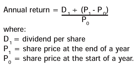
Suppose that a dividend of 5p per share was paid during the year on a share whose value was 100p at the start of the year and 117p at the end of the year:

The total return is made up of a 5% dividend yield and a 17% capital gain. We have just calculated a historical return, on the basis that the dividend income and the price at the end of year one is known. However, calculating the future expected return is a lot more difficult because we will need to estimate both next year ’s dividend and the share price in one year ’s time. Analysts normally consider the different possible returns in alternate market conditions and try and assign a probability to each. The table in Example 1 shows the calculation of the expected return for A plc. The current share price of A plc is 100p and the estimated returns for next year are shown. The investment in A plc is risky. Risk refers to the possibility of the actual return varying from the expected return, ie the actual return may be 30% or 10% as opposed to the expected return of 20%.
REQUIRED RETURN
The required return consists of two elements, which are:
Required return =
Risk-free return + Risk premium
Risk-free return
The risk-free return is the return required by investors to compensate them for investing in a risk-free investment. The risk-free return compensates investors for inflation and consumption preference, ie the fact that they are deprived from using their funds while tied up in the investment. The return on treasury bills is often used as a surrogate for the risk-free rate.
Risk premium
Risk simply means that the future actual return may vary from the expected return. If an investor undertakes a risky investment he needs to receive a return greater than the risk-free rate in order to compensate him. The more risky the investment the greater the compensation required. This is not surprising and it is what we would expect from risk- averse investors.

The Barclay Capital Equity Gilt Study 2003
The Barclay Capital Study calculated the average return on treasury bills in the UK from 1900 to 2002 as approximately 6%. It also calculated that the average return on the UK stock market over this period was 11%. Thus if an investor had invested in shares that had the same level of risk as the market, he would have to receive an extra 5% of return to compensate for the mark et risk. Thus 5% is the historical average risk premium in the UK.
Suppose that Joe believes that the shares in A plc are twice as risky as the market and that the use of long-term averages are valid. The required return may be calculated as follows:
Required = Risk free + Risk
return of A plc return premium
16% = 6% + (5% × 2)
Thus 16% is the return that Joe requires to compensate for the perceived level of risk in A plc, ie it is the discount rate that he will use to appraise an investment in A plc.
THE NPV CALCULATION
Suppose that Joe is considering investing £100 in A plc with the intention of selling the shares at the end of the first year. Assume that the expected return will be 20% at the end of the first year. Given that Joe requires a return of 16% should he invest?
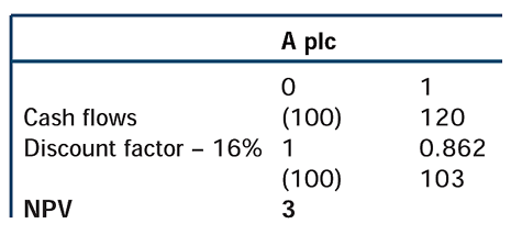
Decision criteria: accept if the NPV is zero or positive. The NPV is positive, thus Joe should invest. A positive NPV opportunity is where the expected return more than compensates the investor for the perceived level of risk, ie the expected return of 20% is greater than the required return of 16%. An NPV calculation compares the expected and required returns in absolute terms.
Calculation of the risk premium
Calculating the risk premium is the essential component of the discount rate. This in turn makes the NPV calculation possible. To calculate the risk premium, we need to be able to define and measure risk.
THE STUDY OF RISK
The definition of risk that is often used in finance literature is based on the variability of the actual return from the expected return. Statistical measures of variability are the variance and the standard deviation (the square root of the variance). Returning to the example of A plc, we will now calculate the variance and standard deviation of the returns.
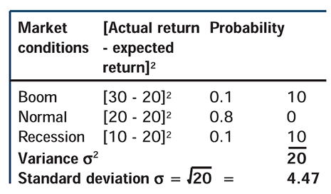
The variance of return is the weighted sum of squared deviations from the expected return. The reason for squaring the deviations is to ensure that both positive and negative deviations contribute equally to the measure of variability. Thus the variance represents ‘rates of return squared’. As the standard deviation is the square root of the variance, its units are in rates of return. As it is easier to discuss risk as a percentage rate of return, the standard deviation is more commonly used to measure risk. In the exam it is unlikely that you will be asked to undertake these basic calculations. The exam questions normally provide you with the expected returns and standard deviations of the returns.
Shares in Z plc have the following returns and associated probabilities:
Probability Return %
0.1 35
0.8 20
0.1 5
Let us then assume that there is a choice of investing in either A plc or Z plc, which one should we choose? To compare A plc and Z plc, the expected return and the standard deviation of the returns for Z plc will have to be calculated.
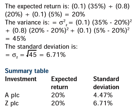
Given that the expected return is the same for both companies, investors will opt for the one that has the lowest risk, ie A plc. The decision is equally clear where an investment gives the highest expected return for a given level of risk. However, these only relate to specific instances where the investments being compared either have the same expected return or the same standard deviation. Where investments have increasing levels of return accompanied by increasing levels of standard deviation, then the choice between investments will be a subjective decision based on the investor’s attitude to risk.
RISK AND RETURN ON TWO-ASSET PORTFOLIOS
So far we have confined our choice to a single investment. Let us now assume investments can be combined into a two-asset portfolio. The risk-return relationship will now be measured in terms of the portfolio’s expected return and the portfolio’s standard deviation.
The following table gives information about four investments: A plc, B plc, C plc, and D plc. Assume that our investor, Joe has decided to construct a two-asset portfolio and that he has already decided to invest 50% of the funds in A plc. He is currently trying to decide which one of the other three investments into which he will invest the remaining 50% of his funds. See Example 2.
The expected return of a two-asset portfolio
The expected return of a portfolio (Rport) is simply a weighted average of the expected returns of the individual investments.
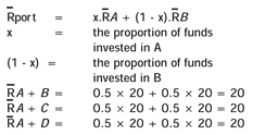
Given that the expected return is the same for all the portfolios, Joe will opt for the portfolio that has the lowest risk as measured by the portfolio’s standard deviation.
The standard deviation of a two-asset portfolio
We can see that the standard deviation of all the individual investments is 4.47%. Intuitively, we probably feel that it does not matter which portfolio Joe chooses, as the standard deviation of the portfolios should be the same (because the standard deviations of the individual investments are all the same).
However, the above analysis is flawed, as the standard deviation of a portfolio is not simply the weighted average of the standard deviation of returns of the individual investments but is generally less than the weighted average. So what causes this reduction of risk? What is the missing factor? The missing factor is how the returns of the two investments co-relate or co-vary, ie move up or down together. There are two ways to measure covariability. The first method is called the covariance and the second method is called the correlation coefficient. Before we perform these calculations let us review the basic logic behind the idea that risk may be reduced depending on how the returns on two investments co -vary.
Portfolio A+B – perfect positive correlation
The returns of A and B move in perfect lock step, (when the return on A goes up to 30%, the return on B also goes up to 30%, when the return on A goes down to 10%, the return on B also goes down to 10%), ie they move in the same direction and by the same degree. See Example 3.
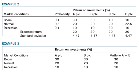
This is the most basic possible example of perfect positive correlation, where the forecast of the actual returns are the same in all market conditions for both investments and thus for the portfolio (as the portfolio return is simply a weighted average). Hence there is no reduction of risk. The portfolio’s standard deviation under this theoretical extreme of perfect positive correlation is a simple weighted average of the standard deviations of the individual investments: σport (A,B) = 4.47 × 0.5 + 4.47 × 0.5 = 4.47
Portfolio A+C – perfect negative correlation
The returns of A and C move in equal but opposite ways (when the return on A goes up to 30%, the return on C goes down to 10%, when the return on A goes down to 10%, the return on C goes up to 30%). See Example 4.

This is the utopian position, ie where the unexpected returns cancel out against each other resulting in the expected return. If the forecast actual return is the same as the expected return under all market conditions, then the risk of the portfolio has been reduced to zero. This is the only situation where the portfolio’s standard deviation can be calculated as follows: σ port (A,C) = 4.47 × 0.5 - 4.47 × 0.5 = 0
Portfolio A+D – no correlation
The returns of A and D are independent from each other. Sometimes they move together, sometimes they move in opposite directions (when the return on A goes up to 30%, the return on D goes down to 10%, when the return on A goes down to 10%, the return on D also goes down to 10%). See Example 5.

The forecast actual return is the same as the expected return under normal market conditions and almost the same under boom market conditions (20 v 21.25). Therefore, we can say that the forecast actual and expected returns are almost the same in two out of the three conditions. This compares with only one condition when there is perfect positive correlation (no reduction of risk) and all three conditions when there is perfect negative correlation (where risk may be eliminated). Therefore, when there is no correlation between the returns on investments this results in the partial reduction of risk.
Measuring covariability
Covariability can be measured in absolute terms by the covariance or in relative terms by the correlation coefficient.
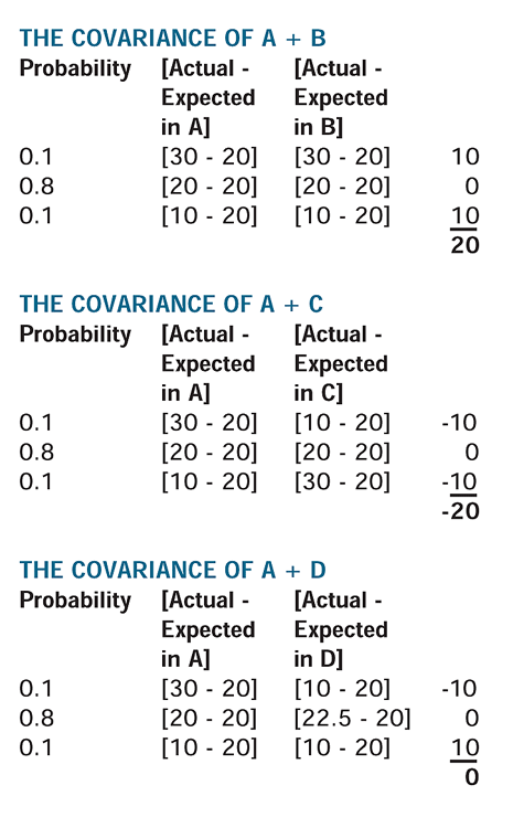
The covariance
For completeness, the calculations of the covariances from raw data are included. However, this approach is not required in the exam, as the exam questions will generally contain the covariances when required.
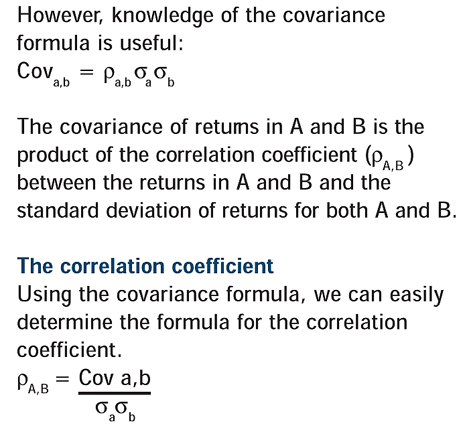
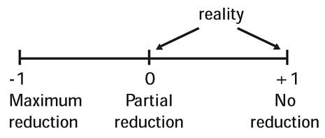
The correlation coefficient as a relative measure of covariability expresses the strength of the relationship between the returns on two investments. It is strictly limited to a range from -1 to +1. See Example 6.
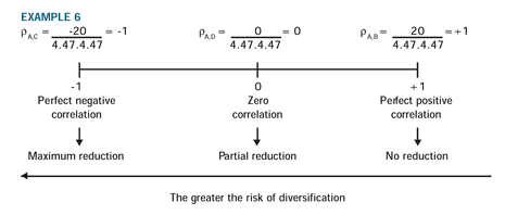
In reality, the correlation coefficient between returns on investments tends to lie between 0 and +1. It is the norm in a two-asset portfolio to achieve a partial reduction of risk (the standard deviation of a two-asset portfolio is less than the weighted average of the standard deviation of the individual investments).
Therefore, we will need a new formula to calculate the risk (standard deviation of returns) on a two -asset portfolio. The formula will obviously take into account the risk (standard deviation of returns) of both investments but will also need to incorporate a measure of covariability as this influences the level of risk reduction.
The formulae for the standard deviation of returns of a two-asset portfolio
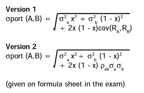
The first two terms deal with the risk of the individual investments. The third term is the most interesting one as it considers the way in which the returns on each pair of investments co-vary. The covariance term is multiplied by twice the proportions invested in each investment, as it considers the covariance of A and B and of B and A, which are of course the same. Note the only difference between the two versions is that the covariance in the second version is broken down into its constituent parts, ie

Based on the first version of the formula:

The second version of the formula is the one that is nearly always used in exams and it is the one that is given on the formula sheet
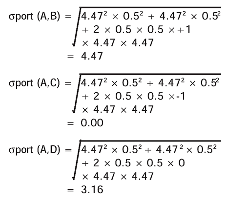
Summary table
Investment Expected Standard
return (%) deviation (%)
Port A + B 20 4.47
Port A + C 20 0.00
Port A + D 20 3.16
A + C is the most efficient portfolio as it has the lowest level of risk for a given level of return.
Perfect negative correlation does not occur between the returns on two investments in the real world, ie risk cannot be eliminated, although it is useful to know the theoretical extremes. However, as already stated, in reality the correlation coefficients between returns on investments tend to lie between 0 and +1. Indeed, the returns on investments in the same industry tend to have a high positive correlation of approximately 0.9, while the returns on investments in different industries tend to have a low positive correlation of approximately 0.2. Thus investors have a preference to invest in different industries thus aiming to create a well- diversified portfolio, ensuring that the maximum risk reduction effect is obtained.
Based on our initial understanding of the risk-return relationship, if investors wish to reduce their risk they will have to accept a reduced return. However, portfolio theory shows us that it is possible to reduce risk without having a consequential reduction in return. This can be proved quite easily, as a portfolio’s expected return is equal to the weighted average of the expected returns on the individual investments, whereas a portfolio’s risk is less than the weighted average of the risk of the individual investments due to the risk reduction effect of diversification caused by the correlation coefficient being less than +1.
We can see from Portfolio A + D above where the correlation coefficient was zero, that by investing in just two investments we can reduce the risk from 4.47% to just 3.16% (a reduction of 1.31 percentage points). Imagine how much risk we could have diversified away, had we created a large portfolio of say 500 different investments or indeed 5,000 different investments.
THE PROOF THAT LARGE PORTFOLIOS INCREASE THE RISK REDUCTION EFFECT
As portfolios increase in size, the opportunity for risk reduction also increases. We are about to review the mathematical proof of this statement. Remember that the SFM paper is not a mathematics paper, so we do not have to work through the derivation of any formulae from first principles. We just need to understand the conclusion of the analysis.
Suppose that we invest equal amounts in a very large portfolio. Then the formula for the variance of the portfolio becomes:

The first term is the average variance of the individual investments and the second term is the average covariance. As N becomes very large the first term tends towards zero, while the second term will approach the average covariance.
In a large portfolio, the individual risk of investments can be diversified away. The individual risk of investments can also be called the specific risk but is normally called the unsystematic risk. However, the risk contributed by the covariance will remain. We already know that the covariance term reflects the way in which returns on investments move together. The returns on most investments will tend to move in the same direction to a greater or lesser degree because of common macro- economic factors affecting all investments. The risk contributed by the covariance is often called the ‘market or systematic risk’. This risk cannot be diversified away.
SYSTEMATIC AND UNSYSTEMATIC RISK
The total risk of a portfolio (as measured by the standard deviation of returns) consists of two types of risk: unsystematic risk and systematic risk. If we have a large enough portfolio it is possible to eliminate the unsystematic risk. However, the systematic risk will remain. See Example 7.
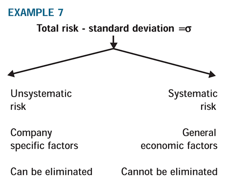
Unsystematic/Specific risk: refers to the impact on a company’s cash flows of largely random events like industrial relations problems, equipment failure, R&D achievements, changes in the senior management team etc. In a portfolio, such random factors tend to cancel as the number of investments in the portfolio increase.
Systematic/Market risk: general economic factors are those macro -economic factors that affect the cash flows of all companies in the stock market in a consistent manner, eg a country’s rate of economic growth, corporate tax rates, unemployment levels, and interest rates. Since these factors cause returns to move in the same direction they cannot cancel out. Therefore, systematic/market risk remains present in all portfolios.
WHAT IS THE IDEAL NUMBER OF INVESTMENTS IN A PORTFOLIO?
Ideally, the investor should be fully diversified, ie invest in every company quoted in the stock market. They should hold the ‘Market portfolio’ in order to gain the maximum risk reduction effect. The good news is that we can construct a well-diversified portfolio, ie a portfolio that will benefit from most of the risk reduction effects of diversification by investing in just 15 different companies in different sectors of the market.
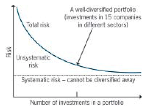
The risk reduction is quite dramatic. We find that two thirds of an investment’s total risk can be diversified away, while the remaining one third of risk cannot be diversified away. A well-diversified portfolio is very easy to obtain, all we have to do is buy a portion of a larger fund that is already well-diversified, like buying into a unit trust or a tracker fund.
Remember that the real joy of diversification is the reduction of risk without any consequential reduction in return. If we assume that investors are rational and risk averse, their portfolios should be well-diversified, ie only suffer the type of risk that they cannot diversify away (systematic risk).
An investor who has a well-diversified portfolio only requires compensation for the risk suffered by their portfolio (systematic risk). Therefore we need to re-define our understanding of the required return:
Required return = Risk free return + Systematic risk premium
Investors who have well-diversified portfolios dominate the market. They only require a return for systematic risk. Thus we can now appreciate the statement ‘that the market only gives a return for systematic risk’.
The next question will be how do we measure an investment’s systematic risk? The answer to this question will be given in the following article on the Capital Asset Pricing Model (CAPM).
10 KEY POINTS TO REMEMBER
1. The expected return on a share consists of a dividend yield and a capital gain/loss in percentage terms.
2. The required return on a risky investment consists of the risk-free rate (which includes inflation) and a risk premium.
3. Total risk is normally measured by the standard deviation of returns ( σ ).
4. Portfolio theory demonstrates that it is possible to reduce risk without having a consequential reduction in return, ie the portfolio’s expected return is equal to the weighted average of the expected returns on the individual investments, while the portfolio risk is normally less than the weighted average of the risk of the individual investments.
5. The extent of the risk reduction is influenced by the way the returns on the investments co-vary. Covariability is normally measured in the exams by the correlation coefficient.
6. In reality, the correlation coefficient between returns on investments tend to lie between 0 and +1. Thus total risk can only be partially reduced, not eliminated.
7 A portfolio’s total risk consists of unsystematic and systematic risk. However, a well-diversified portfolio only suffers from systematic risk, as the unsystematic risk has been diversified away.
8 An investor who holds a well-diversified portfolio will only require a return for systematic risk. Thus their required return consists of the risk-free rate plus a systematic risk premium.
9 Investors who have well-diversified portfolios dominate the market. Thus the market only gives a return for systematic risk.
10 The preparation of a summary table and the identification of the most efficient portfolio (if possible) is an essential exam skill.