Two related articles (Data analytics – parts 1 and 2 – see 'Related links' box) have looked at the way organisations can use data analytics to help understand and manage performance, including the use of predictive analytics to help improve forecasting. This article looks at some important techniques which could be used in forecasting. You should already be familiar with these techniques from your Performance Management (PM) studies, and you should be prepared to apply them to the scenarios in APM questions as necessary.
Forecasting and uncertainty
The business landscape has become increasingly unpredictable and uncertain in recent times due to rapid changes in technology and fierce competition, as well as major global events such as COVID-19.
This uncertainty also makes it increasingly difficult for businesses to budget and forecast accurately. For example, think about the range of factors which could impact a sales forecast:
- Economic conditions (eg economic growth rates, inflation)
- Industry conditions (eg market growth rates, competitors entering/ leaving the market, competitors’ actions)
- The organisation’s products or services (eg whether any new products/services are being launched, or new product features; where products/services are in their life cycle, and whether sales are growing or declining)
- Policy changes (eg changes in the prices of an organisation’s products/services; changes in terms and conditions offered to customers)
- Marketing and advertising (eg increasing/decreasing) advertising activities; launching new marketing campaigns; marketing on new channels)
- Legislation and regulation (eg new legislation - either affecting the organisation’s product, or competitor’s/substitute products)
A comprehensive sales forecast needs to consider all these factors though.
In a previous technical article – Data analytics, part 1 – we highlighted the potential value of predictive analytics in helping organisations understand future patterns and trends, which in turn should help organisations improve the accuracy of their forecasts. Continuing the illustration of sales forecasts, using machine learning-based analytics software which incorporates as rich a data set as possible – including details about external events and market conditions, product life cycles and product launches, historical growth and sales figures, customer surveys and feedback – should help an organisation to improve the accuracy of its sales forecast.
Although the focus of Advanced Performance Management (APM) exam questions will not be on the detailed calculations which would take place in analytics software, accountants need the business knowledge and commercial acumen to interpret the results of data analytics; including having an understanding of the modelling assumptions, and what decisions can justifiably be made based on the analysis.
As such, in the APM exam, you could be expected to draw on analysis techniques to help you understand the assumptions being used in a given scenario, and to evaluate how realistic or plausible they are. You should already be familiar with these techniques from your studies of Performance Management (PM) and Management Accounting (MA), but we are going to briefly recap four techniques which you might need to use in the context of assessing forecasts, or helping to make decisions based on them:
- Regression and correlation
- Time series
- Expected values
- Standard deviation
For the detailed articles relating to each of these teachings, see the following links:
Regression and correlation
Being able to understand the relationship between different factors is very important in forecasting. Regression analysis is a common method used in predictive analytics, where algorithms are trained to understand (or ‘learn’) the relationship between independent variables and a dependent variable. The model can then forecast future trends or product outcomes from new data. For example, in a sales environment, an organisation could use machine learning analytics to predict the next week’s sales, taking account of a number of input factors.
Regression is a technique for investigating the relationship between a dependent variable and an independent variable (or a series of independent variables). The most common form is linear regression, which establishes a linear relationship between two variables, based on a line of best fit.
Regression analysis uncovers the associations between variables. The degree of association is measured by the correlation coefficient (denoted by ‘r’) and is measured on a scale from +1 to -1. When one variable increases as the other increases, the correlation is positive; conversely, if one variable decreases as the other increases, the correlation is negative. The closer the value is to 1 or -1, the stronger the correlation.
A related calculation is the coefficient of determination (calculated as r2). The coefficient of determination identifies the proportion of changed in the dependent variable, which can be explained by changes in the independent variable.
However, it is important to remember that just because two events correlate, this doesn’t necessarily mean that one causes the other.
WORKED EXAMPLE
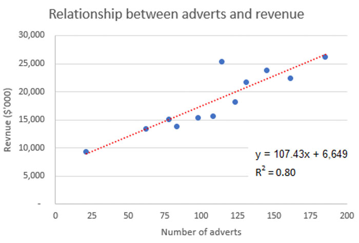
Neen Co has identified there is a positive correlation between the amount of advertising it does in a given period and its revenue in that period. Neen Co’s management accountant has analysed the number of adverts per month in the last year compared to monthly revenue and produced a line of best fit based on this.
Neen Co expects to place 120 adverts in the next month, and the CFO has asked you, using the information prepared by the management accountant, to forecast sales for the next month, but to note any concerns you have about the forecast.

The regression analysis has identified that the line of best fit between the advertising (the independent variable; ‘x’) and revenue (the dependent variable; ‘y’) is calculated as:
y = 107.43x + 6,649.
Using this, we can calculate revenue for the next month as: (107.43 × 120) + 6,649 = $19,541k.
However, in this scenario, r2 = 0.80, meaning that 80% of the changes in revenue can be explained by changes in advertising. This also means that 20% of the changes are due to other factors.
There was a notable outlier in the last year, where the number of adverts was around 115 – relatively close to the number of adverts forecast for the next month (120) – where revenue was slightly above $25 million. The linear model would have predicted revenue of slightly over $19 million [(107.43 × 115) + 6,649 = $19,003k]. This reinforces that there are other factors which could influence revenue, not just the number of adverts.
This links back to the opening illustration at the start of the article, about the range of factors which could influence a sales forecast. Similarly, predictive analytics software takes account of a range of factors when calculating forecasts, reinforcing the point that it would be unrealistic to assume that sales can be accurately forecast on the basis of one independent variable only.
Time series forecasting
Linear regression, which we have just discussed, analyses the relationship between variables using a ‘line of best fit’; that is, a linear trend line.
However, using this type of simple linear relationship alone as the basis of forecasts will not be realistic if there are seasonal variations within the data. In such circumstances, time series analysis can be used to establish not only underlying trends but also seasonal variations within the data. The trend and seasonal variations can then be used together to help make predictions about the future.
ILLUSTRATIVE EXAMPLE
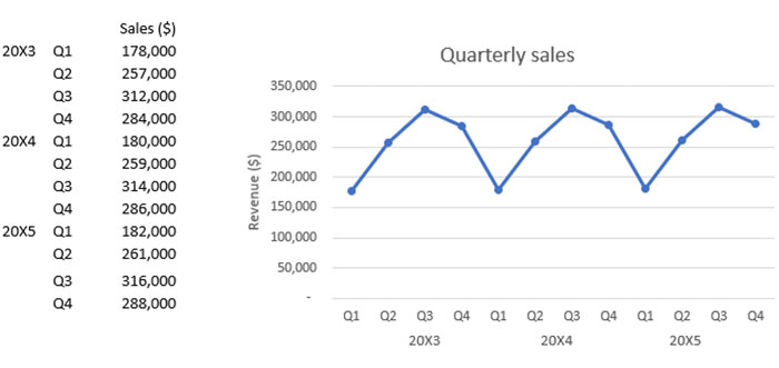
Jeps Co is an events and hospitality company, whose business is highly seasonal. The quarterly sales figures for 20X3 – 20X5 are:

The CFO has asked for a forecast for the sales figures for the first quarter of 20X6.
The assistant management accountant has begun this work. Using moving averages, they calculated that the underlying trend as +$500 per quarter, but the last moving average the assistant calculated was for 20X5 Quarter 2: $261,500.
The assistant has also calculated that the seasonal adjustments for Q1 are either -$79,000 (using an additive model) or 0.70 (using a multiplicative model).
Forecast for 20X6 Qtr 1
The last moving average calculated was 20X5 Qtr 2, which is three periods ago.
So the underlying trend value for 20X6 Qtr 1 will be: $261,500 + (500 × 3) = $263,000.
We then have to adjust for the seasonal variation.
Additive: 263,000 – 79,000 = $184,000
Multiplicative: 263,000 * 0.70 = $184,100
However, as with any forecasts, care needs to be taken when using time series analysis, because it is based on the assumption that the past is a good indicator of what will happen in the future. In our simple example, we have assumed that the underlying sales revenue will continue to grow by $500 per quarter. However, changes in the external and competitive environment can create uncertainty, making forecasts based on past observations unrealistic.
Similarly, effective forecasting relies on the ability to identify genuine patterns and trends in the data. Therefore, analysts need to be able to identify the difference between random fluctuations or outliers and can separate them from underlying trends or seasonal variations.
Expected values
An important aspect of predictive analytics is that it doesn’t simply forecast possible future outcomes it also identifies the likelihood of those events happening.
The availability of information regarding the probabilities of potential outcomes allows the calculation of an expected value for the outcome.
The expected value indicates the expected financial outcome of a decision. It is calculated by multiplying the value associated with each potential outcome by its probability, and then summing the answers.
Expected values can be useful to evaluate alternative courses of action. When making a decision that could have multiple outcomes, a business should look at the value of each alternative and choose the one which has the most beneficial expected value (ie the highest expected value when looking at sales or income; or the lowest expected value when looking at costs).
WORKED EXAMPLE
Mewbix is launching a new cereal product in Deeland, a country with 10 million households.
Mewbix has already introduced the product in some test areas across the country, and - in conjunction with a marketing consultancy business – has been monitoring sales and market share. This data has been supplemented by survey-based tracking of consumer awareness, repeat purchase patterns, and customer satisfaction ratings.
Key findings from the test market and the subsequent customer research have indicated two feasible selling prices for Mewbix: $2.50 or $3.00 per packet. The market research has suggested that, for the coming year:
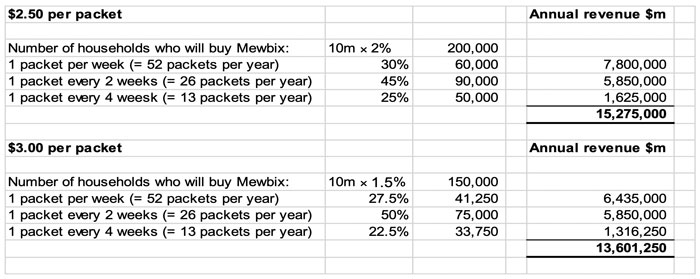
If the selling price is $2.50 per packet, 2% of the households in Deeland will buy Mewbix. Of these, 30% are expected to purchase 1 packet per week, 45% are expected to purchase 1 packet every 2 weeks, and 25% are expected to purchase 1 packet every 4 weeks.
If the selling price is $3.00 per packet, 1.5% of the households will buy Mewbix. Of these 25% are expected to purchase 1 packet per week, 50% are expected to purchase 1 packet every 2 weeks, and 25% are expected to purchase 1 packet every 4 weeks.
Based on the findings from the test market and the subsequent customer research, Mewbix’s CEO has asked for your advice about what price to sell the new cereal for, and how much revenue he should forecast for it in next year’s budget.
In order to give your advice, you need to forecast the revenue expected at each price:

The forecast data suggests that demand for the new cereal is elastic, such that using the higher price leads to a significantly lower annual revenue. As such, the cereal should be sold for $2.50 per packet, and sales of $15,275,000 should be budgeted for the coming year.
However, as with any predictive models, there is no guarantee that the actual sales will mirror the expected values.
Standard deviation
When analysing data sets, it can often be useful to calculate the average (mean) value, to help get a representative estimate for the values in the data set. However, looking at an average value could be misleading when the distribution of values in the dataset is skewed, or when the distribution contains outliers.
Therefore, when looking at average values, it is also important to consider the standard deviation in the dataset.
Standard deviation measures how clustered or dispersed a data set is in relation to its mean.
A low standard deviation tells us that data is clustered around the mean, and therefore the data is accurately characterised by its mean. Conversely, a high standard deviation indicates data is more spread out, such that the mean may not accurately represent the data set. As such, the average is a less reliable indicator of the individual values in a data set where the standard deviation is high, compared to a situation where the standard deviation is low.
WORKED EXAMPLE
Customers who have stayed at Hotel Vaykance, are encouraged to complete a survey, rating how much they have enjoyed their stay on a scale from 1 – 5, with 1 being ‘Not enjoyed at all’ and 5 being ‘Enjoyed greatly’. The surveys then ask further questions, helping management understand why customers have awarded the score they have.
The ‘Average satisfaction score’ is a key performance indicator (KPI) for the business, and is reported in the monthly management information. The KPI reported in last month’s management information was 2.84.
The standard deviation was 1.9, but the standard deviation figure isn’t currently included in the management information. However, the CFO has asked for standard deviation to be included going forwards.
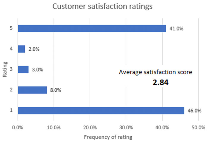
The results from the last month’s customer satisfaction surveys are summarised in the graph below.

The CFO has asked you to explain the significance of standard deviation when assessing the results.
The average satisfaction score (2.84) suggests that customers are reasonably well satisfied with their stay. However, this does not accurately reflect the population, which was polarised between guests who either enjoyed their stay very much (41% at ‘5’) or not at all (46% at ‘1’). The graph showing the results from the customer results survey illustrates this polarisation very clearly.
The standard deviation also highlights this polarisation. A standard deviation of +/- 1.9 compared to an average of 2.84 is very high.
In a scenario like this, where scores were only given between 1 and 5, the highest standard deviation possible would be 2 (ie if 50% of respondents had given a customer satisfaction rating of 5, and 50% had given a rating of 1, the average would be 3, but the standard deviation would be 2). The actual standard deviation of 1.9 is very close to this theoretical maximum, meaning it is very high.
The high standard deviation implies that a large proportion of the dataset is far away from the mean, and therefore it is risky to draw conclusions using the mean.
Written by a member of the APM examining team


